LFQ-DDA QC Peptide-level quantification and summarisation to protein-level abundance

Label-Free Quantification (LFQ) is the simplest form of quantitative proteomics, in which different samples are quantified in separate MS runs. Quantification is either performed by Data-Dependent Aquisition (DDA), where the Mass Spectrometer triggers fragmentation of ions within a given m/z range with the aim being to focus attention of individual peptides separately, or Data-Independent Aquisition (DIA), where a much wider m/z range is used and a mix of peptides are co-fragmented and quantified simultaneously by deconvoluting the resultant complex spectra. Here, we will focus on just LFQ-DDA.

Since each sample is run separately, different peptides will be quantified in each sample and the peptide intensities may not be directly comparable between samples. The common solution to the higher burden of missing values is to use the ‘match-between-runs’ (Cox et al. 2014[UPDATE REF!!!]), or the functionally equivalent ‘Minora’ algorithm employed by Proteome Discoverer (PD). These algorithms use the observed retention times of MS1 ions which were successfully spectrum matched in one sample to identify the likely peptide sequence of MS1 ions that could not be spectrum matched in another sample. However, even with these algorithms, DDA LFQ will still typically have many more missing values than labelled LFQ, e.g TMT.

Despite the pitfalls of LFQ, the data analysis is still relatively straightforward, though there are steps that need some careful consideration and quality control assessment.

Load required packages

To clarify which functionality is provided by which package, we will use package::function. For your own code, there is no need to specify the package unless you want to maintain this clarity.

library(QFeatures)
library(biomasslmb)
library(ggplot2)
library(tidyr)
library(dplyr)

Defining the contaminant proteins

We need to remove contaminant proteins. These were defined here using the cRAP database. Below, we parse the contaminants fasta to extract the IDs for the proteins in both ‘cRAP’ format and Uniprot IDs.


crap_fasta_inf <- system.file(
  "extdata", "cRAP_20190401.fasta.gz", 
  package = "biomasslmb"
)

# Extract the protein IDs associated with each cRAP protein
crap_accessions <- biomasslmb::get_crap_fasta_accessions(crap_fasta_inf)

print(head(crap_accessions))
#> [1] "cRAP001" "P00330"  "cRAP002" "P02768"  "cRAP003" "P00883"

Read in input data

We start by reading in quantitative proteomics data into a QFeatures object, which is the standard Bioconductor object for holding quantitative proteomics data. See here for documentation about the QFeatures object.In this case, we are not adding any experimental details to the QFeatures object, so the ColData will be empty.

?? is a data set available from the biomasslmb package

lfq_dda_pd_PeptideGroups.txt is a file available from the biomasslmb package containing the Peptide-level output from Proteome Discoverer (PD) for an experiment with 6 samples. It is a truncated file containing the precursors peptides quantification for just 500 proteins.

pep_inf <- system.file(
  "extdata", "lfq_dda_pd_PeptideGroups.txt", 
  package = "biomasslmb"
)

Inspecting the column names for the abundances, we see the names are not particularly useful. The Abundance.FXX.na.Sample. part is irrelevant and the replicate number is not included

infdf <- read.delim(pep_inf)

abundance_cols_ix <-18:23

colnames(infdf)[abundance_cols_ix]
#> [1] "Abundance.F12.na.Sample.A" "Abundance.F13.na.Sample.A"
#> [3] "Abundance.F14.na.Sample.A" "Abundance.F15.na.Sample.B"
#> [5] "Abundance.F16.na.Sample.B" "Abundance.F17.na.Sample.B"

Below, we update the column names for the abundance columns

# Clean up sample names
colnames(infdf)[abundance_cols_ix] <- paste(gsub('Abundance.F\\d+.na.Sample.', '',
                                        colnames(infdf)[abundance_cols_ix]), rep(1:3, times=2), sep='_')

colnames(infdf)[abundance_cols_ix]
#> [1] "A_1" "A_2" "A_3" "B_1" "B_2" "B_3"

Before we read in the data, we also want to define the experimental conditions for each sample. We can then provide the

exp_design <- data.frame(quantCols=colnames(infdf)[abundance_cols_ix]) %>%
  separate(quantCols, sep='_', into=c('condition', 'replicate'), remove = FALSE) 

knitr::kable(exp_design)

quantCols	condition	replicate
A_1	A	1
A_2	A	2
A_3	A	3
B_1	B	1
B_2	B	2
B_3	B	3

Now we can read the data into a QFeatures object

# Read in PSM-level quantification from TMT experiment (using QFeatures function)
lfq_qf <- readQFeatures(assayData = infdf,
                        quantCols = abundance_cols_ix, 
                        colData = exp_design,
                        name = "peptides_raw")
#> Checking arguments.
#> Loading data as a 'SummarizedExperiment' object.
#> Formatting sample annotations (colData).
#> Formatting data as a 'QFeatures' object.

Adding the colData to the peptide-level data too.

colData(lfq_qf[['peptides_raw']]) <- colData(lfq_qf)

Extract the gene name and long-form protein name from the descriptions.


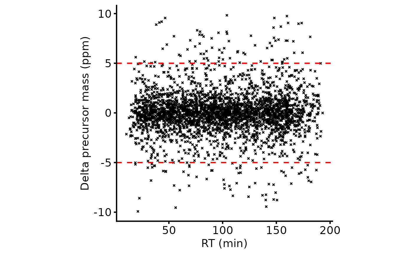
tmt_qf[['peptides_raw']] <- add_gene_long_protein_name_pd(tmt_qf[['peptides_raw']])

It’s helpful to assess the retention time (RT) for the peptides and the relationship with the delta mass for the precursor ion. Everything looks OK here.

plot_rt_dist(lfq_qf[['peptides_raw']])
plot_rt_vs_delta(lfq_qf[['peptides_raw']])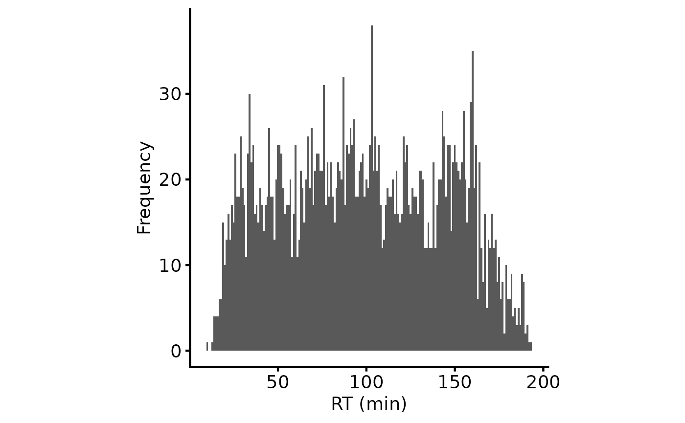

Filter peptides

We first perform routine filtering to remove PSMs that:

Could originate from contaminants. See ?filter_features for further details, including the removal of ‘associated cRAP’.
Don’t have a unique master protein
Don’t have any quantification values

# Perform routine raw data filtering.
# - Remove PSMs from contaminant proteins
# - Remove PSMs where protein ID is empty or not unique

lfq_qf[['peptides_filtered']] <- filter_features_pd_dda(lfq_qf[['peptides_raw']],
                                                        protein_col='Master.Protein.Accessions', # UPDATE WHEN RE-EXPORTED
                                                 contaminant_proteins=crap_accessions,
                                                 filter_contaminant =TRUE,
                                                 filter_associated_contaminant=TRUE,
                                                 unique_master=FALSE,
                                                 remove_no_quant = TRUE)
#> Filtering data...
#> 3106 features found from 500 master proteins => Input
#> 242 contaminant proteins supplied
#> 15 proteins identified as 'contaminant associated'
#> 3091 features found from 498 master proteins => contaminant features removed
#> 3091 features found from 498 master proteins => associated contaminant features removed
#> 3091 features found from 498 master proteins => features without a master protein removed
#> 2746 features found from 461 master proteins => features without quantification removed

We will also remove peptides that are not rank 1 according to the search engine


lfq_qf <- lfq_qf %>%
filterFeatures(~ Search.Engine.Rank.by.Search.Engine.Sequest.HT == 1,
               i = "peptides_filtered") 
#> 'Search.Engine.Rank.by.Search.Engine.Sequest.HT' found in 2 out of 2 assay(s).

biomasslmb:::message_parse(rowData(lfq_qf[['peptides_filtered']]),
                           'Master.Protein.Accessions',
                           "Removing peptides that are not rank 1")
#> 2741 features found from 461 master proteins => Removing peptides that are not rank 1

For the normalisation and summarisation, we need our quantification values to be on a log-scale, so we log-transform below

lfq_qf[['peptides_filtered']] <- QFeatures::logTransform(
  lfq_qf[['peptides_filtered']], base=2)

Next, we plot the peptide intensities.


# Plot the peptide-level quantification distributions per sample
plot_quant(lfq_qf[['peptides_filtered']], log2transform=FALSE, method='density') +
  scale_colour_manual(values=rep(get_cat_palette(3), each=3)) +
  aes(linetype=sample) +
  scale_linetype_manual(values=rep(1:3, times=3)) +
  xlab('Peptide abundance (log2)')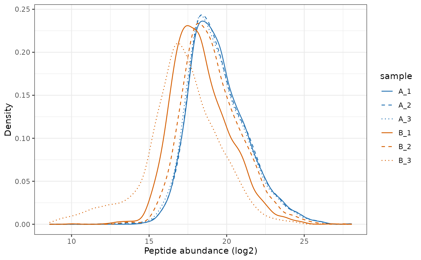

Normalise

Since the same amount of sample was injected for each sample, we want to normalise to remove differences in the overall disribution of abundances. We will thus perform ‘diff.median’ normalisation with QFeatures::normalize.

lfq_qf[['peptides_norm']] <- QFeatures::normalize(lfq_qf[['peptides_filtered']],
                                                  method='diff.median')


# Plot the peptide-level quantification distributions per sample
plot_quant(lfq_qf[['peptides_norm']], log2transform=FALSE, method='density') +
  scale_colour_manual(values=rep(get_cat_palette(3), each=3)) +
  aes(linetype=sample) +
  scale_linetype_manual(values=rep(1:3, times=3)) +
  xlab('Peptide abundance (log2)')

Summarising to protein-level abundances

For the summarisation to protein, we will use robustSummary. We do not need to remove peptides with any missing values. However, we still don’t want to retain peptides with too many missing values, since these will not be very informative in estimating the protein-level quantification.

Below, we inspect the most common patterns for the missing values.

The missingness is most frequently consigned to all samples from one condition and also commonly 2/3 replicates from one condition. It looks like the missingness is far from missing at random (MAR) and is likely missing due to falling below detection limits.

plot_missing_upset(lfq_qf, i='peptides_norm')
#> Warning: `aes_string()` was deprecated in ggplot2 3.0.0.
#> ℹ Please use tidy evaluation idioms with `aes()`.
#> ℹ See also `vignette("ggplot2-in-packages")` for more information.
#> ℹ The deprecated feature was likely used in the UpSetR package.
#>   Please report the issue to the authors.
#> This warning is displayed once every 8 hours.
#> Call `lifecycle::last_lifecycle_warnings()` to see where this warning was
#> generated.
#> Warning: Using `size` aesthetic for lines was deprecated in ggplot2 3.4.0.
#> ℹ Please use `linewidth` instead.
#> ℹ The deprecated feature was likely used in the UpSetR package.
#>   Please report the issue to the authors.
#> This warning is displayed once every 8 hours.
#> Call `lifecycle::last_lifecycle_warnings()` to see where this warning was
#> generated.
#> Warning: The `size` argument of `element_line()` is deprecated as of ggplot2 3.4.0.
#> ℹ Please use the `linewidth` argument instead.
#> ℹ The deprecated feature was likely used in the UpSetR package.
#>   Please report the issue to the authors.
#> This warning is displayed once every 8 hours.
#> Call `lifecycle::last_lifecycle_warnings()` to see where this warning was
#> generated.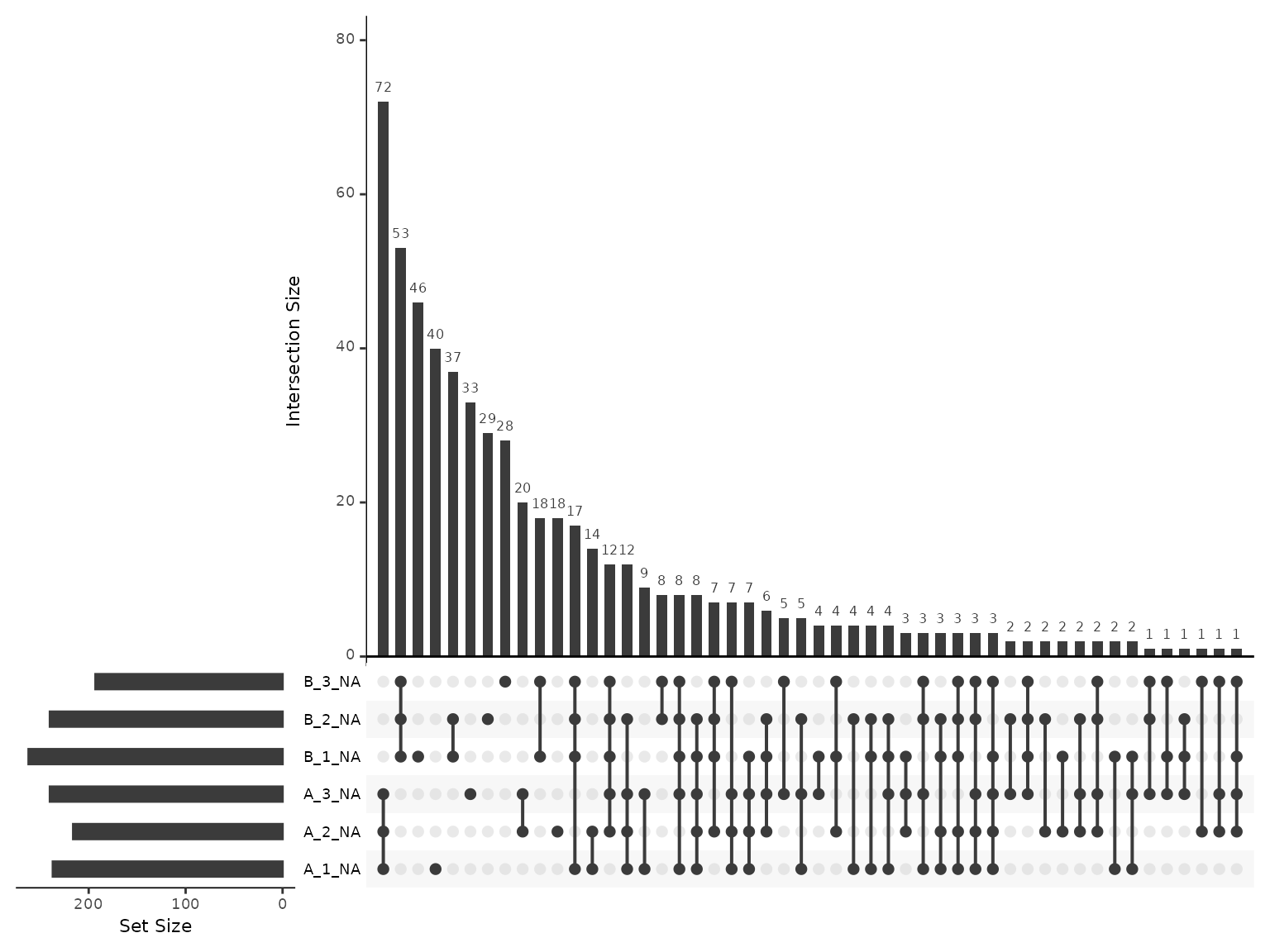

Since DDA LFQ typically has too many missing values to exclude peptides with missing values, the MsCoreUtils::robustSummary method should preferred for summarisation to protein-level abundance. With robustSummary, we do not need to remove all PSMs with missing values since the summarisation algorithm deals with them appropriately (Sticker et al. 2020).. However, we still don’t want to retain PSMs with too many missing values, since these will not be very informative in estimating the protein-level quantification. Here, we will retain PSMs with at most 4/6 missing values


lfq_qf[['peptides_filtered_missing']] <- QFeatures::filterNA(
  lfq_qf[['peptides_norm']], 4/6)

biomasslmb:::message_parse(rowData(lfq_qf[['peptides_filtered_missing']]),
                           'Master.Protein.Accessions',
                           "Removing peptides with more than 4/6 missing values")
#> 2704 features found from 457 master proteins => Removing peptides with more than 4/6 missing values

Next, we remove peptides for proteins with fewer than 2 peptides.

min_peps <- 2
lfq_qf[['peptides_for_summarisation']] <- filter_features_per_protein(
  lfq_qf[['peptides_filtered_missing']], min_features = min_peps)

biomasslmb:::message_parse(rowData(lfq_qf[['peptides_for_summarisation']]),
                           'Master.Protein.Accessions',
                           "Removing 'one-hit' wonders")
#> 2586 features found from 339 master proteins => Removing 'one-hit' wonders

Now we can summarise with robustSummary

set.seed(42)

# Aggregate to protein-level abundances (using QFeatures function)
lfq_qf <- aggregateFeatures(lfq_qf, 
                            i = "peptides_for_summarisation",
                            #i = "peptides_filtered_missing", 
                            fcol = "Master.Protein.Accessions",
                            name = "protein",
                            fun = MsCoreUtils::robustSummary,
                            maxit=10000)
#> Your quantitative and row data contain missing values. Please read the
#> relevant section(s) in the aggregateFeatures manual page regarding the
#> effects of missing values on data aggregation.

Prior to summaristaion, we removed PSMs from proteins with fewer than 2 peptides. However, since we left in peptides with missing values, it’s possible for some protein-level abundances to be derived from just a single peptide. We can use the get_protein_no_quant_mask from biomasslmb to identify where the protein abundances will be derived from fewer than n features (peptides). We can then give this mask to mask_protein_level_quant to replace these quantification values with NA.

# plot = TRUE means we will also get a plot of the number of proteins quantified in each sample
protein_retain_mask <- biomasslmb::get_protein_no_quant_mask(
  lfq_qf[['peptides_for_summarisation']], min_features=min_peps, plot=TRUE) 

lfq_qf[['protein']] <- biomasslmb::mask_protein_level_quant(
  lfq_qf[['protein']], protein_retain_mask)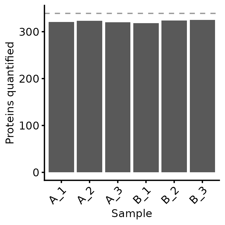

Re-inspecting missing values at protein-level

Now that we have protein-level abundances, we would like to re-inspect the missing values. Overall, we have 5.064 % missing values, with at most 10.565 % missing values in any given sample. The most common missingness patterns are for the protein to be missing from 1,2 or 3 replicates from a single condition, suggesting the quantification is missing due to detection limits.


plot_missing_upset(lfq_qf, i='protein' )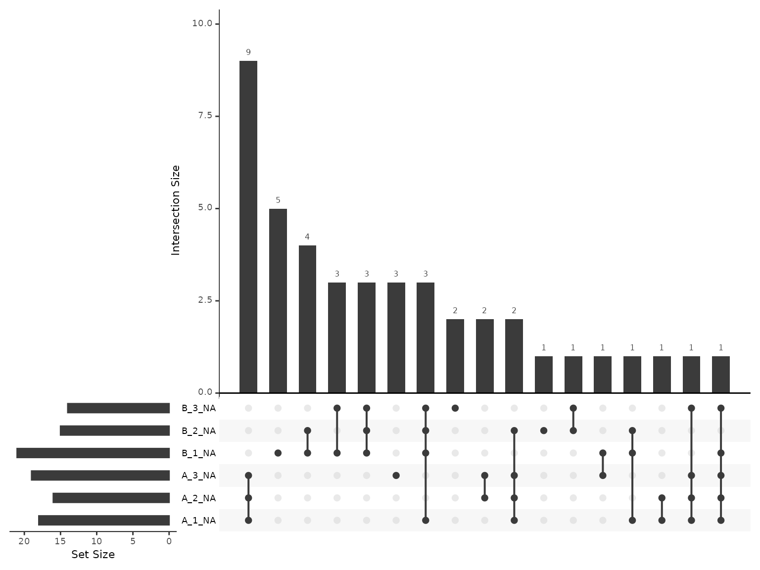

Inspecting the number of peptides and proteins through the processing steps

Now that we have performed all the filtering steps and summarisation to protein-level abundances, it’s helpful to visualise how many peptides/proteins were retained at each level of the processing. We can use the biomasslmb::get_samples_present and biomasslmb::plot_samples_present functions for this. First though, we need to decide which ‘experiments’ we want to plot and define a named character vector since the QFeatures names are not sufficiently clear by themselves

Below, we inspect the experiment names.

names(lfq_qf)
#> [1] "peptides_raw"               "peptides_filtered"         
#> [3] "peptides_norm"              "peptides_filtered_missing" 
#> [5] "peptides_for_summarisation" "protein"

In this case, we don’t want to plot the peptides_norm, since that’s just the normalised quantification present in peptides_filtered and no peptides were removed in that step.

Samples per peptide

We’ll start by inspecting the number of peptides in each experiment. We therefore define a named character vector all the peptides-level experiments, excluding psms_filtered_norm. We set the row variables to be Annotated.Sequence and Modifications so that we count the number of unique peptides.



rename_cols <- c('All peptides' = 'peptides_raw' ,
                 'Quantified, contaminants removed' = 'peptides_filtered',
                 'No missing values' = 'peptides_filtered_missing',
                 '>1 PSM per protein' = 'peptides_for_summarisation')

rowvars <- c('Annotated.Sequence', 'Modifications')

samples_present <- get_samples_present(lfq_qf[,,unname(rename_cols)], rowvars, rename_cols)
#> Warning: 'experiments' dropped; see 'drops()'
#> harmonizing input:
#>   removing 12 sampleMap rows not in names(experiments)
#> Warning in lifeCycle("longForm", package = "MultiAssayExperiment", title = "longFormat"): 'longFormat' is deprecated.
#>   Use 'longForm' instead.
#>   See help('longFormat-deprecated').
plot_samples_present(samples_present, rowvars, breaks=seq(2,10,2)) + ylab('PSM')
#> Scale for fill is already present.
#> Adding another scale for fill, which will replace the existing scale.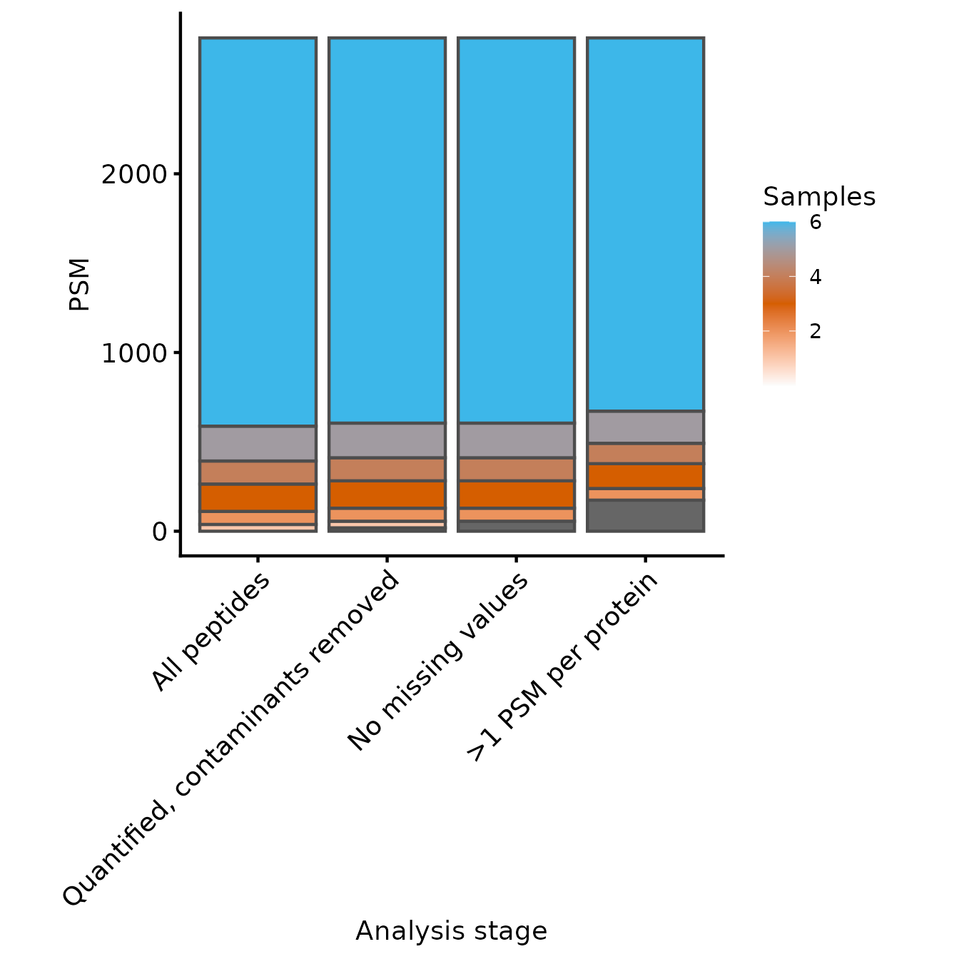

Samples quantified for each PSM at each level of processing

Samples per Protein

Next, we’ll use the same functions to inspect the number of proteins at each level of processing. We need to supply an updated named character vector to include the protein experiment and set the row variables to be just the Master.Protein.Accesions column.


rename_cols_prot <- c(rename_cols, 'Protein'='protein')

rowvars_prot <- c('Master.Protein.Accessions')

samples_present <- get_samples_present(lfq_qf, rowvars_prot, rename_cols_prot)
#> Warning in lifeCycle("longForm", package = "MultiAssayExperiment", title = "longFormat"): 'longFormat' is deprecated.
#>   Use 'longForm' instead.
#>   See help('longFormat-deprecated').
plot_samples_present(samples_present, rowvars_prot, breaks=seq(2,10,2))
#> Scale for fill is already present.
#> Adding another scale for fill, which will replace the existing scale.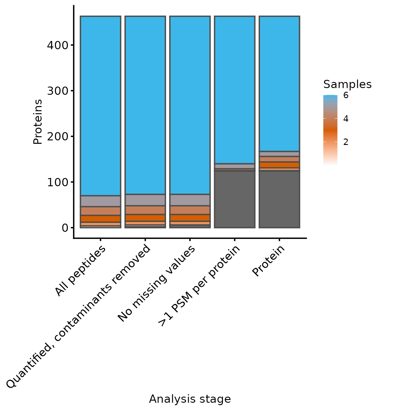

Samples quantified for each protein at each level of processing

From these two plots, we can see that the filtering to ensure that all proteins have >1 peptides removed only a few peptides, but more proteins. Whether this is appropriate will depend on your data in hand.

sessionInfo()
#> R version 4.5.1 (2025-06-13)
#> Platform: x86_64-pc-linux-gnu
#> Running under: Ubuntu 24.04.3 LTS
#> 
#> Matrix products: default
#> BLAS:   /usr/lib/x86_64-linux-gnu/openblas-pthread/libblas.so.3 
#> LAPACK: /usr/lib/x86_64-linux-gnu/openblas-pthread/libopenblasp-r0.3.26.so;  LAPACK version 3.12.0
#> 
#> locale:
#>  [1] LC_CTYPE=C.UTF-8       LC_NUMERIC=C           LC_TIME=C.UTF-8       
#>  [4] LC_COLLATE=C.UTF-8     LC_MONETARY=C.UTF-8    LC_MESSAGES=C.UTF-8   
#>  [7] LC_PAPER=C.UTF-8       LC_NAME=C              LC_ADDRESS=C          
#> [10] LC_TELEPHONE=C         LC_MEASUREMENT=C.UTF-8 LC_IDENTIFICATION=C   
#> 
#> time zone: UTC
#> tzcode source: system (glibc)
#> 
#> attached base packages:
#> [1] stats4    stats     graphics  grDevices utils     datasets  methods  
#> [8] base     
#> 
#> other attached packages:
#>  [1] dplyr_1.1.4                 tidyr_1.3.1                
#>  [3] ggplot2_4.0.0               biomasslmb_0.0.4           
#>  [5] QFeatures_1.18.0            MultiAssayExperiment_1.34.0
#>  [7] SummarizedExperiment_1.38.1 Biobase_2.68.0             
#>  [9] GenomicRanges_1.60.0        GenomeInfoDb_1.44.3        
#> [11] IRanges_2.42.0              S4Vectors_0.46.0           
#> [13] BiocGenerics_0.54.1         generics_0.1.4             
#> [15] MatrixGenerics_1.20.0       matrixStats_1.5.0          
#> 
#> loaded via a namespace (and not attached):
#>  [1] DBI_1.2.3               gridExtra_2.3           rlang_1.1.6            
#>  [4] magrittr_2.0.4          clue_0.3-66             compiler_4.5.1         
#>  [7] RSQLite_2.4.3           png_0.1-8               systemfonts_1.3.1      
#> [10] vctrs_0.6.5             reshape2_1.4.4          stringr_1.5.2          
#> [13] ProtGenerics_1.40.0     pkgconfig_2.0.3         crayon_1.5.3           
#> [16] fastmap_1.2.0           backports_1.5.0         XVector_0.48.0         
#> [19] labeling_0.4.3          rmarkdown_2.30          UCSC.utils_1.4.0       
#> [22] UpSetR_1.4.0            visdat_0.6.0            ragg_1.5.0             
#> [25] purrr_1.1.0             bit_4.6.0               xfun_0.53              
#> [28] cachem_1.1.0            jsonlite_2.0.0          blob_1.2.4             
#> [31] DelayedArray_0.34.1     cluster_2.1.8.1         R6_2.6.1               
#> [34] bslib_0.9.0             stringi_1.8.7           RColorBrewer_1.1-3     
#> [37] genefilter_1.90.0       jquerylib_0.1.4         Rcpp_1.1.0             
#> [40] knitr_1.50              usethis_3.2.1           BiocBaseUtils_1.10.0   
#> [43] Matrix_1.7-3            splines_4.5.1           igraph_2.2.1           
#> [46] tidyselect_1.2.1        abind_1.4-8             yaml_2.3.10            
#> [49] lattice_0.22-7          tibble_3.3.0            plyr_1.8.9             
#> [52] withr_3.0.2             KEGGREST_1.48.1         S7_0.2.0               
#> [55] evaluate_1.0.5          uniprotREST_1.0.0       desc_1.4.3             
#> [58] survival_3.8-3          Biostrings_2.76.0       pillar_1.11.1          
#> [61] corrplot_0.95           checkmate_2.3.3         rprojroot_2.1.1        
#> [64] scales_1.4.0            xtable_1.8-4            glue_1.8.0             
#> [67] lazyeval_0.2.2          tools_4.5.1             robustbase_0.99-6      
#> [70] annotate_1.86.1         fs_1.6.6                XML_3.99-0.19          
#> [73] grid_4.5.1              MsCoreUtils_1.20.0      AnnotationDbi_1.70.0   
#> [76] GenomeInfoDbData_1.2.14 naniar_1.1.0            cli_3.6.5              
#> [79] textshaping_1.0.4       S4Arrays_1.8.1          AnnotationFilter_1.32.0
#> [82] gtable_0.3.6            DEoptimR_1.1-4          sass_0.4.10            
#> [85] digest_0.6.37           SparseArray_1.8.1       htmlwidgets_1.6.4      
#> [88] farver_2.1.2            memoise_2.0.1           htmltools_0.5.8.1      
#> [91] pkgdown_2.1.3           lifecycle_1.0.4         httr_1.4.7             
#> [94] bit64_4.6.0-1           MASS_7.3-65

Sticker, Adriaan, Ludger Goeminne, Lennart Martens, and Lieven Clement. 2020. “Robust Summarization and Inference in Proteome-wide Label-free Quantification.” Molecular & cellular proteomics: MCP 19 (7): 1209–19. https://doi.org/10.1074/mcp.RA119.001624.

Tom Smith

2025-10-29