LFQ-DIA QC Peptide-level quantification and summarisation to protein-level abundance

THIS VIGNETTE IS A WORK IN PROGRESS!

Label-Free Quantification (LFQ) is the simplest form of quantitative proteomics, in which different samples are quantified in separate MS runs. Quantification is either performed by Data-Dependent Aquisition (DDA), where the Mass Spectrometer triggers fragmentation of ions within a given m/z range with the aim being to focus attention of individual peptides separately, or Data-Independent Aquisition (DIA), where a much wider m/z range is used and a mix of peptides are co-fragmented and quantified simultaneously by deconvoluting the resultant complex spectra. Here, we will focus on just LFQ-DIA.

MORE DETAILS ON DIA REQUIRED HERE!

Load required packages

To clarify which functionality is provided by which package, we will use package::function. For your own code, there is no need to specify the package unless you want to maintain this clarity.

library(QFeatures)
library(biomasslmb)
library(ggplot2)
library(tidyr)
library(dplyr)

Defining the contaminant proteins

We need to remove contaminant proteins. These were defined here using the cRAP database. Below, we parse the contaminants fasta to extract the IDs for the proteins in both ‘cRAP’ format and Uniprot IDs.


crap_fasta_inf <- system.file(
  "extdata", "cRAP_20190401.fasta.gz", 
  package = "biomasslmb"
)

# Extract the protein IDs associated with each cRAP protein
crap_accessions <- biomasslmb::get_crap_fasta_accessions(crap_fasta_inf)

print(head(crap_accessions))
#> [1] "cRAP001" "P00330"  "cRAP002" "P02768"  "cRAP003" "P00883"

Read in input data

We start by reading in quantitative proteomics data into a QFeatures object, which is the standard Bioconductor object for holding quantitative proteomics data. See here for documentation about the QFeatures object.

Here, we will use the biomasslmb::readDIANNFilter function, which also allows us to control the FDR thresholds for the precursor and protein (run-specific and global). This function reads in the report.tsv file from DIA-NN. If you are happy with the filtering settings in DIA-NN, you can directly read the report.pr_matrix.tsv into a QFeatures object using the QFeatures::readQFeatures function.

diann_report.tsv is a file available from the biomasslmb package containing the output from DIA-NN for an experiment with 6 samples. It is a truncated file containing the precursors (peptides) for just 500 proteins.

diann_report_inf <- system.file(
  "extdata", "diann_report.tsv", 
  package = "biomasslmb"
)

dia_qf <- readDIANNFilterQJoin(diann_report_inf,
                               global_protein_q=0.01,
                               run_protein_q=0.01,
                               run_precursor_q=0.01)
#> Checking arguments.
#> Loading data as a 'SummarizedExperiment' object.
#> Splitting data in runs.
#> Formatting sample annotations (colData).
#> Formatting data as a 'QFeatures' object.
#> Setting assay rownames.
#> 'Lib.PG.Q.Value' found in 6 out of 6 assay(s).
#> 'PG.Q.Value' found in 6 out of 6 assay(s).
#> 'Q.Value' found in 6 out of 6 assay(s).
#> Warning: 'experiments' dropped; see 'drops()'
#> harmonizing input:
#>   removing 6 sampleMap rows not in names(experiments)

We have 0 quantification values which are exactly zero here. Where these do exist, they should be replaced with NA, since mass spectrometry is not capable of asserting that the protein had zero abundance in the sample.

tmt_qf[['peptides_fdr_cntrl']] <- QFeatures::zeroIsNA(dia_qf[['peptides_fdr_cntrl']])

Our column names include redundant information (‘HYE_DIA’)

colnames(dia_qf)[["peptides_fdr_cntrl"]]
#> [1] "HYE_DIA_A1" "HYE_DIA_A2" "HYE_DIA_A3" "HYE_DIA_B1" "HYE_DIA_B2"
#> [6] "HYE_DIA_B3"

Below, we update the column names to remove the redundant information and then update the sample names in the QFeatures

colnames(dia_qf)[["peptides_fdr_cntrl"]] <- gsub('HYE_DIA_', '', colnames(dia_qf)[["peptides_fdr_cntrl"]])
dia_qf <- renamePrimary(dia_qf, colnames(dia_qf)[["peptides_fdr_cntrl"]])

We need to populate the colData, which is currently empty

data.frame(colData(dia_qf))
#> data frame with 0 columns and 6 rows

Here, we can create our colData from the sample names. In other cases, you may need to read in a separate experimental design file.


colData(dia_qf) <- data.frame(quantCols=rownames(colData(dia_qf))) %>%
  separate(quantCols, sep='', into=c(NA, 'condition', 'replicate'), remove = FALSE) %>%
  tibble::column_to_rownames('quantCols')

data.frame(colData(dia_qf))
#>    condition replicate
#> A1         A         1
#> A2         A         2
#> A3         A         3
#> B1         B         1
#> B2         B         2
#> B3         B         3

Adding the colData to the peptide-level data too.

colData(dia_qf[['peptides_fdr_cntrl']]) <- colData(dia_qf)

We first perform routine filtering to remove PSMs that:

Could originate from contaminants. See ?filter_features_pd_dda for further details, including the removal of ‘associated cRAP’.
Don’t have a unique master protein.

dia_qf[['peptides_filtered']] <- biomasslmb::filter_features_diann(dia_qf[['peptides_fdr_cntrl']], contaminant_proteins=crap_accessions)
#> Filtering data...
#> 5009 features found from 454 master proteins => Input
#> 242 contaminant proteins supplied
#> 11 proteins identified as 'contaminant associated'
#> 4998 features found from 453 master proteins => contaminant features removed
#> 4998 features found from 453 master proteins => associated contaminant features removed
#> 4998 features found from 453 master proteins => features without a master protein removed
#> 4955 features found from 448 master proteins => features with non-unique master proteins removed
#> 4955 features found from 448 master proteins => features without quantification removed

Check normalisation

Next, we plot the peptide intensity distribution to check they are approximately the same using biomasslmb::plot_quant. By default, DIA-NN performs normalisation. See the documentation for details of the underlying assumptions for the normalisation and use cases where this normalisation approach may not be appropriate, e.g interactome proteomics.


# Plot the peptide-level quantification distributions per sample
biomasslmb::plot_quant(dia_qf[['peptides_filtered']],
                       log2transform=TRUE,
                       method='density') +
  theme_biomasslmb() +
  xlab('PSM abundance (log2)')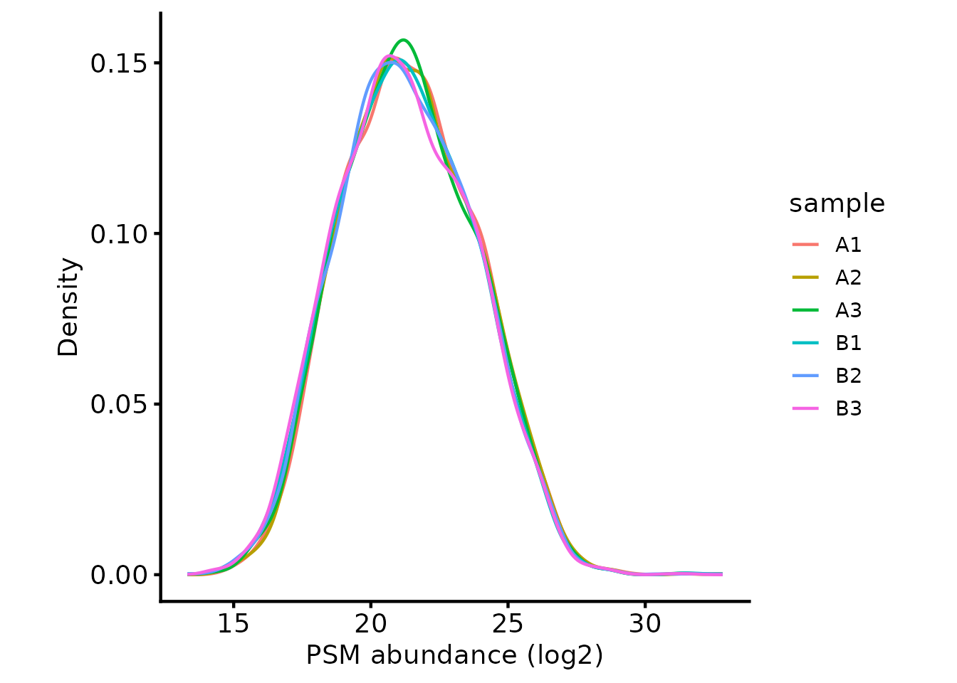

Missing values

Below, we inspect the number of missing values per sample



nNA(dia_qf[['peptides_filtered']])$nNAcols %>%
  data.frame() %>% knitr::kable(digits=2)

name	nNA	pNA
A1	641	0.13
A2	736	0.15
A3	1029	0.21
B1	674	0.14
B2	597	0.12
B3	613	0.12

Here, the samples have between 12 - 21 % missing values. This is fairly typical of DIA data at the precursor level.

Next, we inspect the most common patterns for the missing values.

plot_missing_upset(dia_qf, i='peptides_filtered')
#> Warning: `aes_string()` was deprecated in ggplot2 3.0.0.
#> ℹ Please use tidy evaluation idioms with `aes()`.
#> ℹ See also `vignette("ggplot2-in-packages")` for more information.
#> ℹ The deprecated feature was likely used in the UpSetR package.
#>   Please report the issue to the authors.
#> This warning is displayed once every 8 hours.
#> Call `lifecycle::last_lifecycle_warnings()` to see where this warning was
#> generated.
#> Warning: Using `size` aesthetic for lines was deprecated in ggplot2 3.4.0.
#> ℹ Please use `linewidth` instead.
#> ℹ The deprecated feature was likely used in the UpSetR package.
#>   Please report the issue to the authors.
#> This warning is displayed once every 8 hours.
#> Call `lifecycle::last_lifecycle_warnings()` to see where this warning was
#> generated.
#> Warning: The `size` argument of `element_line()` is deprecated as of ggplot2 3.4.0.
#> ℹ Please use the `linewidth` argument instead.
#> ℹ The deprecated feature was likely used in the UpSetR package.
#>   Please report the issue to the authors.
#> This warning is displayed once every 8 hours.
#> Call `lifecycle::last_lifecycle_warnings()` to see where this warning was
#> generated.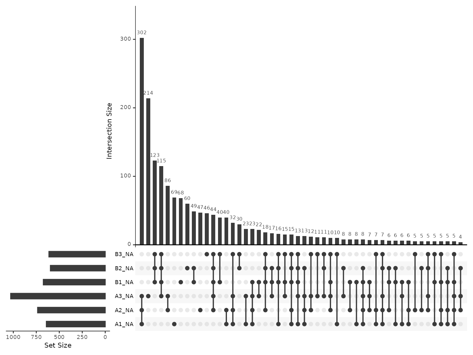

The missingness is frequently observed for all 3 replicates of a single condition, but also commonly just for a single sample.

Summarising to protein-level abundances

Now that we have inspected the peptide-level quantification and filtered the peptides, we can summarise the peptide-level quantification to protein-level abundances.

Since DIA typically has too many missing values to exclude peptides with missing values, the MsCoreUtils::robustSummary method should preferred for summarisation to protein-level abundance. With robustSummary, we do not need to remove all PSMs with missing values since the summarisation algorithm deals with them appropriately (Sticker et al. 2020).. However, we still don’t want to retain PSMs with too many missing values, since these will not be very informative in estimating the protein-level quantification. Here, we will retain PSMs with at most 4/6 missing values

dia_qf[['peptides_filtered_missing']] <- QFeatures::filterNA(
  dia_qf[['peptides_filtered']], 4/6)

biomasslmb:::message_parse(rowData(dia_qf[['peptides_filtered_missing']]),
                           'Protein.Group',
                           "Removing peptides with > 4/6 missing values")
#> 4863 features found from 441 master proteins => Removing peptides with > 4/6 missing values

Next, we will remove PSMs for proteins with fewer than 2 PSMs. This is a common filter in proteomics to ensure the protein-level quantifications are derived from at least two independent observations. In some cases, for example phosphoproteomics, or where this filter appears to be too stringent, it may be appropriate to skip it.


min_psms <- 2
 
dia_qf[['peptides_filtered_forRobust']] <- biomasslmb::filter_features_per_protein(
  dia_qf[['peptides_filtered_missing']], min_features = min_psms, master_protein_col='Protein.Group')

biomasslmb:::message_parse(rowData(dia_qf[['peptides_filtered_forRobust']]),
                           'Protein.Group',
                           "Removing peptides for proteins with < 2 peptides")
#> 4829 features found from 407 master proteins => Removing peptides for proteins with < 2 peptides

Now we can summarise with robustSummary


# Aggregate to protein-level abundances (using QFeatures function)
dia_qf <- QFeatures::aggregateFeatures(dia_qf, 
                                       i = "peptides_filtered_forRobust", 
                                       fcol = "Protein.Group",
                                       name = "protein",
                                       fun = MsCoreUtils::robustSummary,
                                       maxit=10000) # ensure sufficient iterations for convergance
#> Your quantitative data contain missing values. Please read the relevant
#> section(s) in the aggregateFeatures manual page regarding the effects
#> of missing values on data aggregation.

biomasslmb:::message_parse(rowData(dia_qf[['protein']]),
                           'Protein.Group',
                           "Summarised to proteins")
#> 407 features found from 407 master proteins => Summarised to proteins

Prior to summaristaion, we removed PSMs from proteins with fewer than 2 PSMs. However, since we left in PSMs with missing values, it’s possible for some protein-level abundances to be derived from just a single PSM. We can use the get_protein_no_quant_mask from biomasslmb to identify where the protein abundances will be derived from fewer than n features (PSMs). We can then give this mask to mask_protein_level_quant to replace these quantification values with NA.

# plot = TRUE means we will also get a plot of the number of proteins quantified in each sample
protein_retain_mask <- biomasslmb::get_protein_no_quant_mask(
  dia_qf[['peptides_filtered_forRobust']], min_features=2, plot=TRUE, master_protein_col='Protein.Group')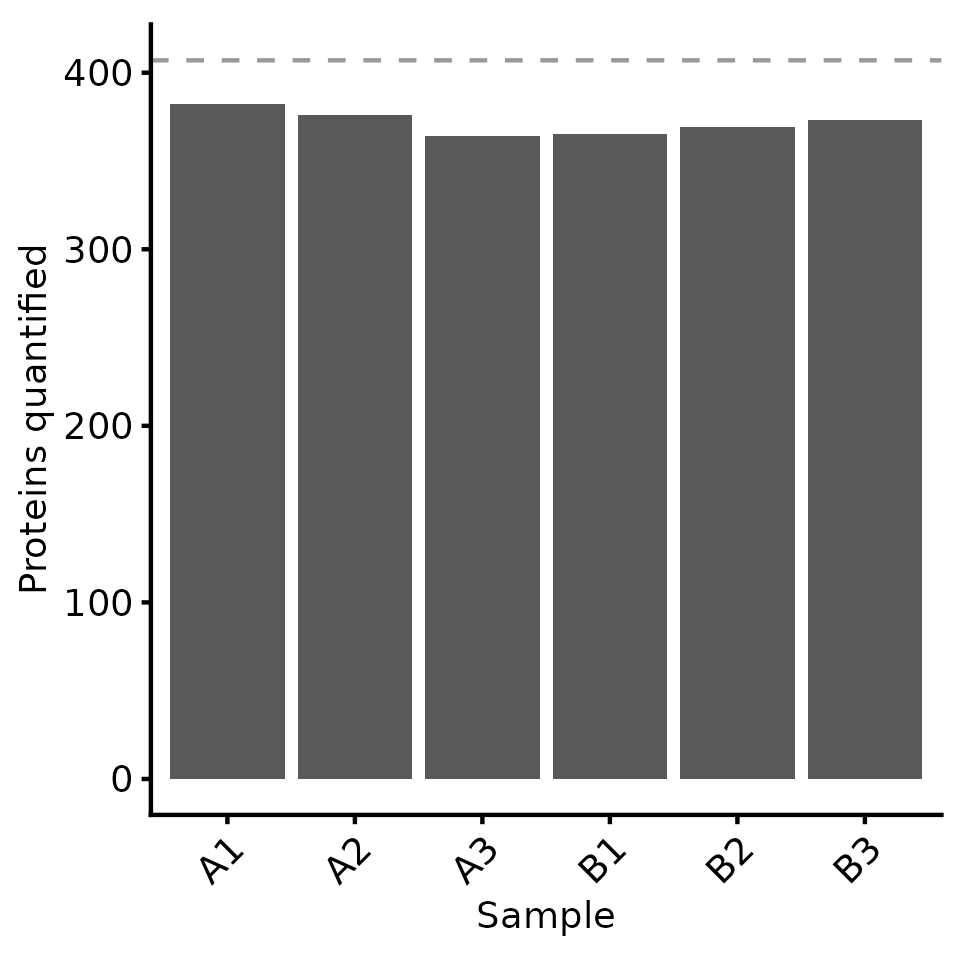


dia_qf[['protein']] <- biomasslmb::mask_protein_level_quant(
  dia_qf[['protein']], protein_retain_mask)

Re-inspecting missing values at protein-level

Now that we have protein-level abundances, we would like to re-inspect the missing values. Overall, we have 8.722 % missing values, with at most 10.565 % missing values in any given sample. The most common missingness pattern is for the protein to be missing from all 3 samples for a single condition.


nNA(dia_qf[['protein']])$nNAcols %>%
  data.frame() %>% knitr::kable(digits=2)

name	nNA	pNA
A1	25	0.06
A2	31	0.08
A3	43	0.11
B1	42	0.10
B2	38	0.09
B3	34	0.08


plot_missing_upset(dia_qf, i='protein')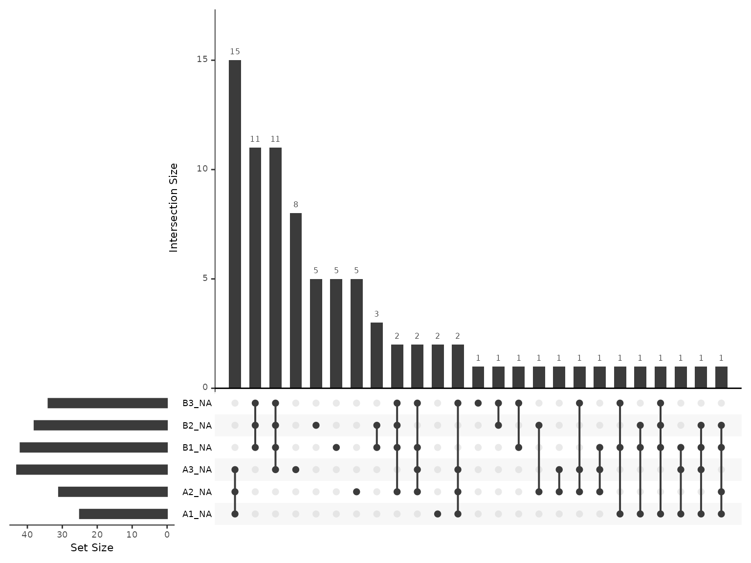

Inspecting the number of peptides and proteins through the processing steps

Now that we have performed all the filtering steps and summarisation to protein-level abundances, it’s helpful to visualise how many peptides/proteins were retained at each level of the processing. We can use the biomasslmb::get_samples_present and biomasslmb::plot_samples_present functions for this. First though, we need to decide which ‘experiments’ we want to plot and define a named character vector since the QFeatures names are not sufficiently clear by themselves

Below, we inspect the experiment names.

names(dia_qf)
#> [1] "peptides_fdr_cntrl"          "peptides_filtered"          
#> [3] "peptides_filtered_missing"   "peptides_filtered_forRobust"
#> [5] "protein"

In this case, we want to plot all the experiments.

Samples per PSM

We’ll start by inspecting the number of PSMs in each experiment. We therefore define a named character vector all the PSM-level experiments, exlcuding psms_filtered_norm. We set the row variables to be Precursor.Id so that we count the number of unique peptides (precursors).




rename_cols <- c('Peptides passing FDR thresholds' = 'peptides_fdr_cntrl' ,
                 'Quantified, contaminants removed' = 'peptides_filtered',
                 '<= 4/6 missing values' = 'peptides_filtered_missing',
                 '>1 peptides per protein' = 'peptides_filtered_forRobust')

rowvars <- c('Precursor.Id')

samples_present <- get_samples_present(dia_qf[,,unname(rename_cols)], rowvars, rename_cols)
#> harmonizing input:
#>   removing 6 sampleMap rows not in names(experiments)
#> Warning in lifeCycle("longForm", package = "MultiAssayExperiment", title = "longFormat"): 'longFormat' is deprecated.
#>   Use 'longForm' instead.
#>   See help('longFormat-deprecated').
plot_samples_present(samples_present, rowvars, breaks=seq(2,10,2)) + ylab('PSM')
#> Scale for fill is already present.
#> Adding another scale for fill, which will replace the existing scale.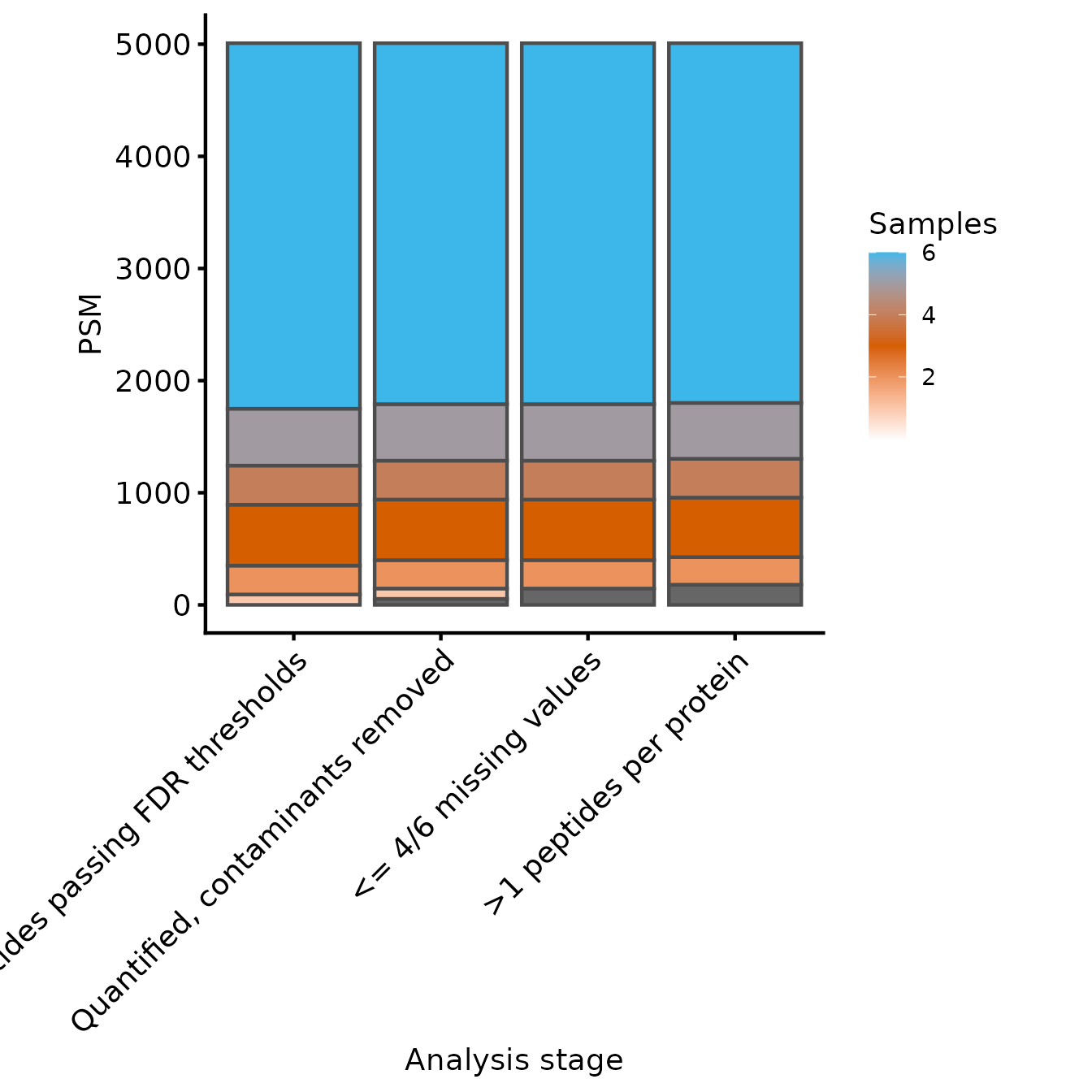

Samples quantified for each PSM at each level of processing

Samples per Protein

Next, we’ll use the same functions to inspect the number of proteins at each level of processing. We need to supply an updated named character vector to include the protein experiment and set the row variables to be just the Master.Protein.Accesions column.


rename_cols_prot <- c(rename_cols, 'Protein'='protein')

rowvars_prot <- c('Protein.Group')

samples_present <- get_samples_present(dia_qf, rowvars_prot, rename_cols_prot)
#> Warning in lifeCycle("longForm", package = "MultiAssayExperiment", title = "longFormat"): 'longFormat' is deprecated.
#>   Use 'longForm' instead.
#>   See help('longFormat-deprecated').
plot_samples_present(samples_present, rowvars_prot, breaks=seq(2,10,2))
#> Scale for fill is already present.
#> Adding another scale for fill, which will replace the existing scale.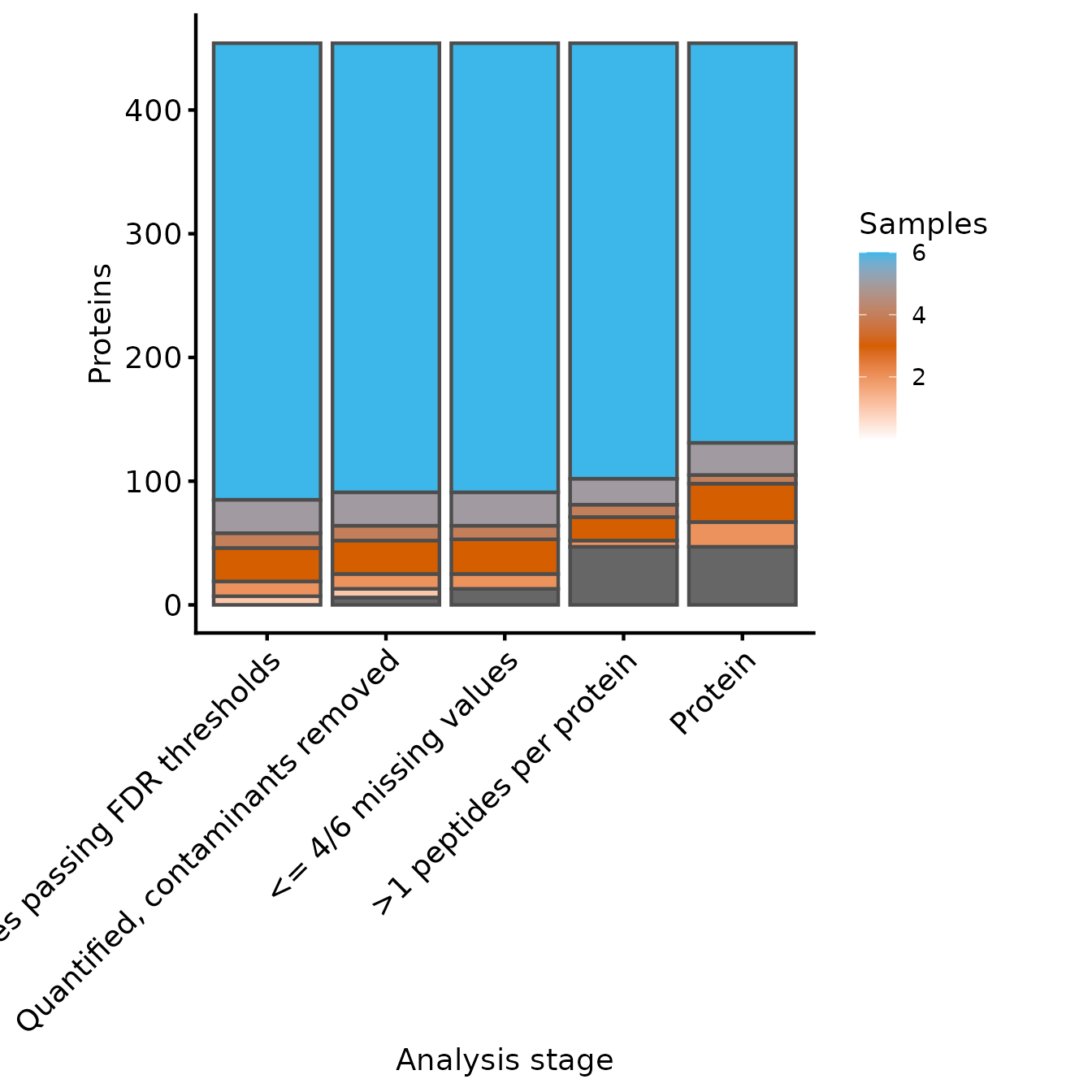

Samples quantified for each protein at each level of processing

From these two plots, we can see that the filtering to ensure that all proteins have >1 peptides removed only a few peptides, but more proteins. Whether this is appropriate will depend on your data in hand.

sessionInfo()
#> R version 4.5.1 (2025-06-13)
#> Platform: x86_64-pc-linux-gnu
#> Running under: Ubuntu 24.04.3 LTS
#> 
#> Matrix products: default
#> BLAS:   /usr/lib/x86_64-linux-gnu/openblas-pthread/libblas.so.3 
#> LAPACK: /usr/lib/x86_64-linux-gnu/openblas-pthread/libopenblasp-r0.3.26.so;  LAPACK version 3.12.0
#> 
#> locale:
#>  [1] LC_CTYPE=C.UTF-8       LC_NUMERIC=C           LC_TIME=C.UTF-8       
#>  [4] LC_COLLATE=C.UTF-8     LC_MONETARY=C.UTF-8    LC_MESSAGES=C.UTF-8   
#>  [7] LC_PAPER=C.UTF-8       LC_NAME=C              LC_ADDRESS=C          
#> [10] LC_TELEPHONE=C         LC_MEASUREMENT=C.UTF-8 LC_IDENTIFICATION=C   
#> 
#> time zone: UTC
#> tzcode source: system (glibc)
#> 
#> attached base packages:
#> [1] stats4    stats     graphics  grDevices utils     datasets  methods  
#> [8] base     
#> 
#> other attached packages:
#>  [1] dplyr_1.1.4                 tidyr_1.3.1                
#>  [3] ggplot2_4.0.0               biomasslmb_0.0.4           
#>  [5] QFeatures_1.18.0            MultiAssayExperiment_1.34.0
#>  [7] SummarizedExperiment_1.38.1 Biobase_2.68.0             
#>  [9] GenomicRanges_1.60.0        GenomeInfoDb_1.44.3        
#> [11] IRanges_2.42.0              S4Vectors_0.46.0           
#> [13] BiocGenerics_0.54.1         generics_0.1.4             
#> [15] MatrixGenerics_1.20.0       matrixStats_1.5.0          
#> 
#> loaded via a namespace (and not attached):
#>  [1] DBI_1.2.3               gridExtra_2.3           rlang_1.1.6            
#>  [4] magrittr_2.0.4          clue_0.3-66             compiler_4.5.1         
#>  [7] RSQLite_2.4.3           png_0.1-8               systemfonts_1.3.1      
#> [10] vctrs_0.6.5             reshape2_1.4.4          stringr_1.5.2          
#> [13] ProtGenerics_1.40.0     pkgconfig_2.0.3         crayon_1.5.3           
#> [16] fastmap_1.2.0           backports_1.5.0         XVector_0.48.0         
#> [19] labeling_0.4.3          rmarkdown_2.30          UCSC.utils_1.4.0       
#> [22] UpSetR_1.4.0            visdat_0.6.0            ragg_1.5.0             
#> [25] purrr_1.1.0             bit_4.6.0               xfun_0.53              
#> [28] cachem_1.1.0            jsonlite_2.0.0          blob_1.2.4             
#> [31] DelayedArray_0.34.1     cluster_2.1.8.1         R6_2.6.1               
#> [34] bslib_0.9.0             stringi_1.8.7           RColorBrewer_1.1-3     
#> [37] genefilter_1.90.0       jquerylib_0.1.4         Rcpp_1.1.0             
#> [40] knitr_1.50              usethis_3.2.1           BiocBaseUtils_1.10.0   
#> [43] Matrix_1.7-3            splines_4.5.1           igraph_2.2.1           
#> [46] tidyselect_1.2.1        abind_1.4-8             yaml_2.3.10            
#> [49] lattice_0.22-7          tibble_3.3.0            plyr_1.8.9             
#> [52] withr_3.0.2             KEGGREST_1.48.1         S7_0.2.0               
#> [55] evaluate_1.0.5          uniprotREST_1.0.0       desc_1.4.3             
#> [58] survival_3.8-3          Biostrings_2.76.0       pillar_1.11.1          
#> [61] corrplot_0.95           checkmate_2.3.3         rprojroot_2.1.1        
#> [64] scales_1.4.0            xtable_1.8-4            glue_1.8.0             
#> [67] lazyeval_0.2.2          tools_4.5.1             robustbase_0.99-6      
#> [70] annotate_1.86.1         fs_1.6.6                XML_3.99-0.19          
#> [73] grid_4.5.1              MsCoreUtils_1.20.0      AnnotationDbi_1.70.0   
#> [76] GenomeInfoDbData_1.2.14 naniar_1.1.0            cli_3.6.5              
#> [79] textshaping_1.0.4       S4Arrays_1.8.1          AnnotationFilter_1.32.0
#> [82] gtable_0.3.6            DEoptimR_1.1-4          sass_0.4.10            
#> [85] digest_0.6.37           SparseArray_1.8.1       htmlwidgets_1.6.4      
#> [88] farver_2.1.2            memoise_2.0.1           htmltools_0.5.8.1      
#> [91] pkgdown_2.1.3           lifecycle_1.0.4         httr_1.4.7             
#> [94] bit64_4.6.0-1           MASS_7.3-65

Sticker, Adriaan, Ludger Goeminne, Lennart Martens, and Lieven Clement. 2020. “Robust Summarization and Inference in Proteome-wide Label-free Quantification.” Molecular & cellular proteomics: MCP 19 (7): 1209–19. https://doi.org/10.1074/mcp.RA119.001624.

Tom Smith

2025-10-29